Variable transformation, configuration of analogue inputs

Each HW data point has value transformation properties. They are used to recalculate the raw value read over the I/O bus to a value which represents the corresponding physical value or written from variable to I/O.

If a transform has to be applied on the client side, for example a value of 1236 to 12.36, the raw value must be divided by 100. The coeficient K of a linear transformation is then 0,01. If this value is read, it is simple and logical. This logic needs to be applied for the writing process as well. If you have value of 12.36 in a program and you want to transform it to 1236 on a communication bus, the value must be divided by 100, and the coeficient is again 0,01. There is no difference between reading and writing here.

For example, a temperature measured by a passive Pt1000 sensor is communicated from the I/O module RCIO as resistance, multiplied by 10 to obtain higher resolution when communicated as INTEGER: for a Pt1000 sensor at 22 °C the communicated value on the I/O bus is 10857, which represents the sensor resistance of 1085.7 Ohm. This value is linearised in the Pt1000 specific linearisation table „resistancetotemperature“, and the output is temperature in °C.

These are the predefined transforms:

• Identity - the value is not transformed, it is brought to the program as is

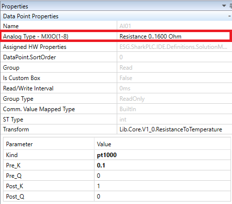
• Resistance to temperature - linearisation curve for Pt100, Pt500, Pt1000, Ni1000-5000, Ni1000-6180 sensors. The transform has following parameters:
  • Kind - sensor type which determines the predefined linearisation curve
  • Pre_K - first linear pre-linearisation transform y = Kx + Q coefficient, should be 0.1 for Domat I/O modules, because resistance is read as Ohm*10
  • Pre_Q - first linear pre-linearisation transform y = Kx + Q coefficient (used for sensor cable resistance compensation)
  • Post_K - second linear post-linearisation transform y = Kx + Q coefficient
  • Post_Q - second linear post-linearisation transform y = Kx + Q coefficient (used for compensation of absolute sensor measuring error in °C)

• Threshold - detector for transform of an analogue value into binary value (if a resistance AI is used as a DI). The transform has following parameters:
  • Threshold - a limit to switch from True to False and back
  • Invert - inverts the function: if Invert = True, the transform output is False if the input value is higher than the Threshold.

• Window - if the input value is between predefined limits, the output is True, otherwise False. Example: damaged sensor detection - if the measured value is lower than -40 °C or higher than 150 °C, the sensor is damaged and the output value is True (using the Invert function)
  • Low - lower limit
  • High - higher limit
  • Invert - inverts the function: if Invert = True then if the value is within limits, the output is False, otherwise it is True.

• LinearByTable - linearisation curve with max. 8 points. The curve is defined using pairs of values - coordinates of the points in X and Y vectors. Input values are in the X vector, the corresponding output values are in the Y vector. The vector is in square brackets, values are separated by commas.
  • XValues - vector with X coordinates of the linearisation curve points
  • YValues - vector with Y coordinates of the linearisation curve points
  • Active points - number of points used, max. 8, taken from the left of the vector
  • Pre_K - first linear pre-linearisation transform y = Kx + Q coefficient
  • Pre_Q - first linear pre-linearisation transform y = Kx + Q coefficient
  • Post_K - second linear post-linearisation transform y = Kx + Q coefficient
  • Post_Q - second linear post-linearisation transform y = Kx + Q coefficient
    

• Negate - for bool type values (DI), negates the input value

• LinearByTwoPoints - a simple linear transform defined by two points. The input range X1…X2 is converted to the output range Y1…Y2. Often used with analog sensors, e.g. input of 0…10 V (0…10 000 mV) is converted to -20…50 °C: X1 = 0, X2 = 10000, Y1 = -20, Y2 = 50.
  • X1 - X coordinate of the first point
  •  X2 - X coordinate of the second point
  • Y1 - Y coordinate of the first point
  • Y2 - Y coordinate of the second point

• LinearWithShiftByTwoPoints - a linear transform defined by two points. The input value can be shifted before transformation by the Shift parameter, the output value may be limited by the Min and Max parameters.
  • Shift - value added to the input before the transform
  • X1 - X coordinate of the first point
  • X2 - X coordinate of the second point
  • Y1 - Y coordinate of the first point
  • Y2 - Y coordinate of the second point
  • Min - low limit for output limitation, the output value is higher than or equal to Min
  • Max - high limit for output limitation, the output value is lower than or equal to Max

• Linear - a simple linear transform defined by y = Kx + Q
  • K - multiplication coefficient
  • Q - addition coefficient
    • For basic conversion of voltage or current to measured physical value, e.g. a 0…50 °C sensor with 0…10 V output has K = 0,005 (voltage is read in mV), Q = 0.

• StaefaT1 - transform for temperature sensors T1 by Staefa Control System
  • Pre_K - first linear pre-linearisation transform y = Kx + Q coefficient, should be 0.1 for Domat I/O modules, because resistance is read as Ohm*10
  • Pre_Q - first linear pre-linearisation transform y = Kx + Q coefficient (used for sensor cable resistance compensation)
  • Post_K - second linear post-linearisation transform y = Kx + Q coefficient
  • Post_Q - second linear post-linearisation transform y = Kx + Q coefficient (used for compensation of absolute sensor measuring error in °C)

• LinearWithShift - a linear transform defined by y = Kx + Q. The input value can be shifted before transformation by the Shift parameter, the output value may be limited by the Min and Max parameters.
  • Shift - value added to the input before the transform
  • K - multiplication coefficient
  • Q - addition coefficient
  • Min - low limit for output limitation, the output value is higher than or equal to Min
  • Max - high limit for output limitation, the output value is lower than or equal to Max

A transform is defined „from the physical inputs to the program (structured text)“, IO→ST - if there is a global variable mapped on a HW variable for writing (hardware analogue output), and a value multiplied by 100 shall be written, e.g. a HVAC integer, a constant of k=0,01 must be entered in the linear transform. This rule is used in other transformations as well. Transformations “LinearByTable” and “LinearByTwoPoints” have parameters X and Y. X stands for values, that are written to output. Y values are values visible in our project.

If a resistance temperature sensor is connected to a physical analogue input of a module, we need to be sure that the correct physical value is measured, and that the correct type of transformation is used.

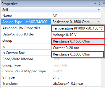
At first, the correct physical value must be chosen on the AI. This can be done by changing “Analog Type - MMIO/MCIO2” property in AI properties. We have three options how to measure temperature with Pt1000 sensor. The first one is to use “Temperature Pt1000 -50..150°C” option. In this case, the linearization would be done in I/O module. However, a recommended solution is to use “Resistance 0..1600Ohm” or “Resistance 0..5000Ohm” option. In this case, the linearization will be done in PLC, on the runtime level.

The next step is to set the correct transformation. To transform resistance to temperature, “ResistanceToTemperature” transformation must be chosen.

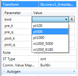
Then select „kind“ as Pt1000. This selects the set of coefficients in the linearisation table automatically. The last step, which is defined by character of AI, is to set variable pre_k to value 0.1. This will modify the input signal before SW transformation. Result of these steps is final value in °C. Resistance 0-1600 Ohm is on AI measured in range 0-16000 (Ohm * 10 for higher resolution), therefore it needs to be divided by 10 before entering the transformation. This setting can be specific for Domat I/O modules only.

The last step is to upload our configuration to the I/O module and to the PLC. Default setting on AI of I/O module is Voltage 0-10V. The AI setting needs to be changed to Resistance 0-1600 Ohm or 0-5000 Ohm. If all AIs are edited as necessary, the solution can be deployed to the PLC. The process of deployment is described in chapter Uploading of a program to a PLC. PLC must be then started in Commissioning mode. In this mode, the IDE is able to communicate directly with I/O modules and change their settings. Settings of Domat modules can be changed by clicking on “Domat - Configure module” option in the context menu of an I/O module.



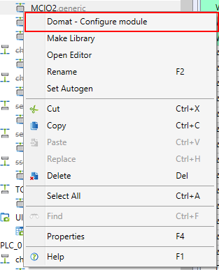
This change will be shown immediately and I/O module does not need to be restarted manually.
The transformation is uploaded with the solution in the process of deployment. If we switch the PLC run mode to “Full run” or “Only communication” mode, all AIs should show correct measured temperature immediately. Remember to restart the PLC as Cold restart.

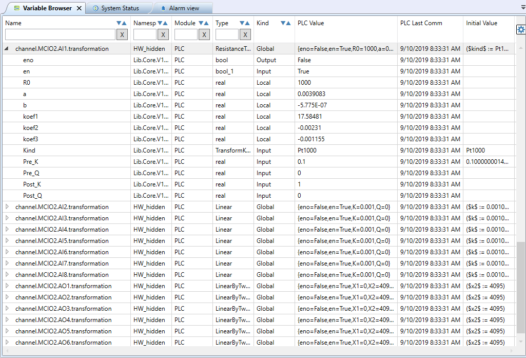
If a transform is used on a data point, such as Lib.Core.v1_0.ResistanceToTemperature, new variables with namespace “hw_hidden” are visible in the Variable Browser after compilation. These variables are not available until the project has been compiled.

Unwrap a “HW hidden” variable to display the parameters of  the transformation in “Channel name”.“Device Name”.“Data Point”.“transformation” (e.g. channel.MCIO2.AI1.transformation). Start debug to watch the real values in the “PLC Value” column, while in the “Initial Value” the preset value in the controller is displayed.

If analog type is changed on a data point, reconfigure the Domat modules accordingly by right click on the device - Domat module configuration. The modules must be online. It is not necessary to deploy the solution to apply the configuration in the module(s).

Successful module reconfiguration is indicated by a dialog.

A mere change of data point transformation parameters does not require reconfiguration of the I/O module. To apply changes, just upload the solution to a PLC, and run PLC with warm restart. The change of parameters can be verified in Debug mode, in Variable Browser at the datapoint with hw_hidden namespace. 

1. Change the transform e.g. from ResistanceToTemperature to another transform, e.g. Linear, upload the solution, and run the PLC with warm restart. Then, change the transform to its original value (from Linear to  ResistanceToTemperature) and configure the temperature sensor type and parameters. After solution upload and warm restart, the new parameters are applied. This way does not require cold restart.
2. In case the project is allowed to be rerun with cold restart, change the parameter, upload the solution, and run the PLC with cold restart. 

Hints and tips when configuring the data points

1. To configure a data point, it is not necessary to rerun the project with cold restart.
2. Reconfiguration of a data point is only required if an analog type has been changed.
3. After changing a transform, only solution upload and warm restart are necessary.
4. In case the project must not be rerun with cold restart (technological reasons) and a parameter change is necessary, proceed according to a) above.